

Experiments
Below are synopses of the 25 experiments in "Physical Experiments in Heat Transfer and Thermodynamics."
A video clip explaining each experiment is included in a CD that is bundled with the book.
Also included on the CD are the Excel data files that go along with each experiment.
Experiment 1
Viscosity of Water as a Function of Temperature – Capillary Tube
This experiment uses a submerged capillary tube (1.715 mm inside diameter) fixed near the bottom of a Styrofoam tank. There is a bell-mouth opening at the tube inlet end, inside the tank. The outlet end of the tube is located just outside the tank. The discharge rate through the tube depends on length, diameter, differential pressure and viscosity, which is dependent on temperature. In an Excel file, data are provided for 19 runs for water temperatures ranging from 0.3°C to 35°C. The results agree nicely with contemporary and historic viscosity curves.
Experiment 2
Viscosity of Water as a Function of Temperature – Rotating Cylinder
The viscosity of water as a function of temperature is obtained with an entirely different apparatus than the capillary tube in Experiment 1. In this experiment our viscometer consists of a fixed outer cylinder and a concentric rotating inner cylinder, with water in the annual gap between the cylinders. The inner cylinder is given an initial spin and the water provides a shear stress that causes the cylinder to coast-down and come to a stop. The rate at which the cylinder slows down is related to the water’s viscosity, which depends on temperature. Water, ranging in temperature from 3°C to 30°C, is tested and the corresponding coast-down data are used to compute the viscosity of water as a function of temperature.
Experiment 3
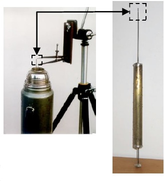
Density of Water in the Neighborhood of 4°C
In this experiment we find the density of water in the neighborhood of 4°C with a sensitive cylindrical float whose diameter is only 1.25 mm at the water line. The float is placed in a Thermos bottle filled with water whose temperature is varied from run-to-run. From 0°C to 4°C (water density is a maximum at 4°C) the float rises about 8 mm, and from 4°C to 25°C the float sinks about 40 mm. The data reduction includes differential and integral calculus to account for thermal expansion of the float. The final results closely follow the published density curve, including the characteristic hump at 4°C.
Experiment 4
Enthalpy of Fusion for Water
The enthalpy of fusion for water, hsf is the energy removed from 0°C liquid water to make 0°C solid ice. In this experiment we use an electrically heated ice calorimeter. The phase change process takes place isothermally at 0°C, so by keeping the surroundings of the calorimeter at this temperature the calorimeter becomes adiabatic during the heating process. The students reduce the data and obtain an hsf 1.5% lower than the published value.
Experiment 5
Specific Heat of Aluminum – Electric Calorimeter
The specific heat of aluminum is found with a differential electric calorimeter that has two individual calorimeters – each an assembly of 13 aluminum plates electrically heated. The exterior surfaces of both calorimeters and the surrounding insulation are identical. However, the
interior plates are different – one calorimeter has solid interior plates
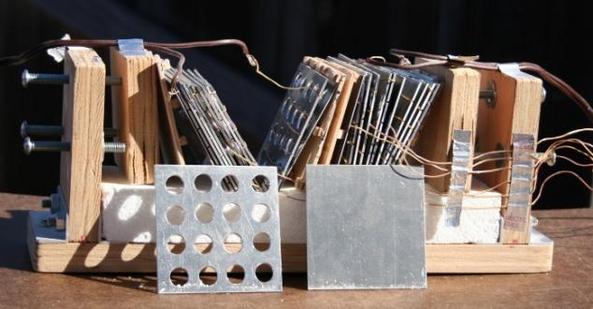
and the other has perforated interior plates, thus the aluminum mass is different. By adjusting the electrical power into each calorimeter the temperature-versus-time curves for each calorimeter are matched. This curve match allows cancellation of the unknown heat loss from each calorimeter. The data reduction scheme includes integral calculus and produces a specific heat value 6.6% lower than the published value.
Experiment 6
Specific Heat of Aluminum - Transient Cooling Calorimeter
The specific heat of aluminum is obtained with an entirely different calorimeter than the one previously described in Experiment 5. In the present experiment the calorimeter is a hollow aluminum cylinder, closed at one end and fitted with an aluminum plug at the other end, forming a watertight cavity. The calorimeter is heated with a hair
drier and then allowed to cool in still air. Two tests are performed: one with water in the cavity and one without water in the cavity. Transient temperature measurements from the two tests, collected with a digital data acquisition system, give different cooling rates characterized with Excel Trendlines. The data reduction is rigorous and includes integral and differential calculus. Three different approaches are used to reduce the same data to obtain the specific heat of aluminum. The average value obtained is 5.6% off the published value.
Experiment 7
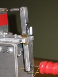
Thermal Expansion of Aluminum
The coefficient of linear thermal expansion for aluminum is obtained with an aluminum welding rod heated in a copper-tube oven. In the oven the welding rod is radially constrained while free to axially expand as the oven temperature increases. The rod’s expansion is measured with a pivoting lever-arm that makes needle contact with one end of the rod. Attached to the lever-arm is a mirror that rotates with the arm and reflects a laser beam that is projected on a laboratory wall. This arrangement provides an elongation amplification ratio of 383:1. Students use the Excel data provided and obtain a final result that is only 0.9% different than the published value.
Experiment 8
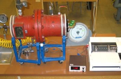
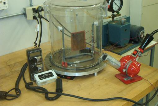
Polytropic Expansion of Air
The expansion or compression of a gas can be described by the polytropic equation pv^n=c where p is pressure, v is specific volume, c is a constant, and the exponent n depends on the thermodynamic process. In our experiment, compressed air in a steel pressure vessel is discharged to the atmosphere while the air remaining inside expands. Transient temperature and pressure measurements of the air inside the vessel are recorded. Students will reduce these data to find the polytropic exponent n for the expansion process and will see that the process Trendline carries a correlation coefficient of 0.9998.
Experiment 9
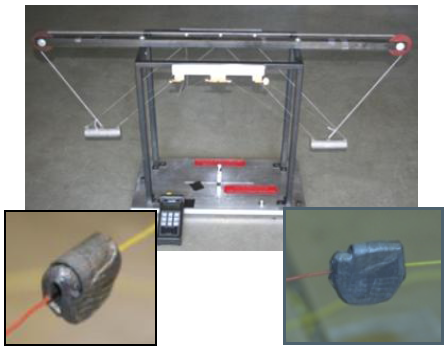
First Law of Thermodynamics – Lead Smashing
The first law of thermodynamics is verified with two steel cylinders smashing a small piece of lead. The elevated cylinders swing as pendulums from opposite directions, simultaneously striking the lead. The loss in gravitational potential energy of the cylinders is equated to the rise in internal energy of the lead. The data are plotted in Excel and fitted with a Trendline. The final result is 0.9% off the published value of Joule’s constant, J = 778 (ft lbf)/Btu. Part of the data reduction includes an uncertainty analysis that is covered in an appendix.
Experiment 10
First Law of Thermodynamics – Friction Bearing
The first law of thermodynamics is verified with a friction bearing experiment. A copper friction bearing is driven in rotation with a falling weight. Friction causes the bearing to heat-up. Data reduction analysis accounts for gravitational potential energy, translational and rotational kinetic energy, internal energy, and heat loss from the bearing. Again, the final result compares very well (1.9%) with the published value of Joule’s constant, J = 778 (ft lbf)/Btu.
Experiment 11
First Law of Thermodynamics – Copper Cold Working
The first law of thermodynamics is verified again, this time with a copper hinge calorimeter that is “cold worked” by a swinging pendulum which causes a rise in the hinge temperature. The loss in potential energy of the pendulum is equated to the rise in internal energy of the hinge, plus the heat unavoidably transferred into the hinge clamps. The final result is a Joule’s constant value that compares well (7.2%) with the published value.

Experiment 12
First Law of Thermodynamics – Bicycle Braking
The first law of thermodynamics is verified yet again – this time with a bicycle. A lever-mounted, copper calorimeter friction pad rubs on the front tire, heats-up, brings the bicycle to a stop, and gives Joule’s constant with a 14% margin of error. Used in the data reduction analysis are aerodynamic drag and rolling friction obtained with bicycle coast-down speeds read into a
cassette audio recorder. These data are fitted with a Trendline and used with an integral and a differential equation in the analysis. This experiment is fun and provides rigorous and instructive data reduction analysis while physically confirming the first law of thermodynamics.
Experiment 13
Vapor-Compression Refrigeration Cycle
Designed and fabricated in-house, this second-generation system has features not found in expensive, commercial, educational equipment. Refrigerant temperatures, pressures, and flow rate are measured throughout the closed loop. With 2.5 m long, calibrated venturi flow meters, air flows through the evaporator and condenser are measured. A speed and torque sensor gives shaft power driving the compressor. The write-up,
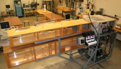
with 16 pages, 17 photos, and 5 illustrations, along with the video, thoroughly explain the entire system. Students use the Excel data to perform a complete thermodynamic analysis including psychrometrics, which is included in the write-up. The data reveal an interesting departure from the standard textbook cycle.
Experiment 14
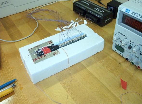
Thermal Conductivity
In this experiment an aluminum rod is heated with an electric-resistance heater on one end, and is cooled by circulating water in a cooling jacket and on the other end. Insulation around the rod (removed from the rod and in the background in the photo) restricts conduction in the axial direction only. Thermocouples are connected to a PC digital data acquisition system. The reduced data give an average thermal conductivity of the aluminum that differs by 5.4% from the published value.
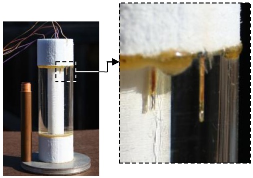
Experiment 15
Thermal Conductivity as a Function of Temperature
Thermal conductivity varies with temperature. This behavior is more pronounced with acrylic than with aluminum. In this experiment we find thermal conductivity as a function of temperature for acrylic. A hollow acrylic cylinder with an imbedded electric heater is placed in an ice water bath. The cylinder ends are well insulated causing the heat to propagate in the radial direction only. Thermocouple temperature measurements and heater electrical power input measurements are recorded with a PC digital data acquisition system. These data are reduced to give the thermal conductivity as a function of temperature.
Experiment 16
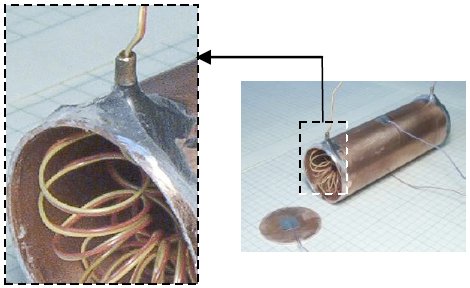
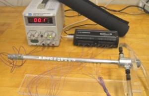
Transient One-Dimensional Conduction
In this experiment an indirect, iterative, numerical method is used to obtain the thermal diffusivity (α) of stainless steel. A stainless steel tube is electrically heated at one end which results in heat diffusing through the remaining length of the tube. Temperatures from ten thermocouples are recorded with a digital data acquisition system at discrete time steps. The system’s governing partial differential equation contains the unknown α and is solved in Excel using boundary condition and initial condition temperatures from the experiment. Students iteratively vary α to match the computed temperature distribution curve with the measured temperature distribution curve. The unknown α is obtained at curve match.
Experiment 17
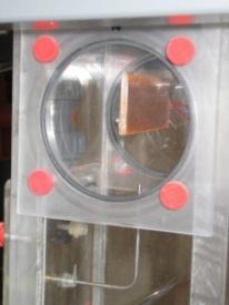
Forced Convection – Flat Plate in Water
In this experiment we use an electrically heated copper plate in a water tunnel which provides forced convection cooling. Water velocity, water and plate temperatures, and electrical power input to the heater are recorded and used to find the convection coefficient. For a range of velocities, two data series are provided: one for water at 2°C (Pr = 12) and one for water at 25°C (Pr = 6). Students use these data and plot the results using so called “primitive variables” which include the convection coefficient, water velocity, and water temperature. This experiment ties-in with the following two experiments.
Experiment 18
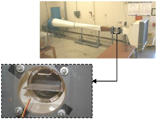
Forced Convection and Radiation – Flat Plate in Air
Two, electrically-heated, aluminum plates are set in a wind tunnel and subjected to forced convection cooling over a range of free stream velocities. In an Excel file two data series are provided: one for a 53 mm long plate and one for a 90 mm long plate. As in the previous experiment (Experiment 17) the results are expressed in primitive variables. In the
experiment that follows (Experiment 19, Data Correlation with Dimensionless Numbers) students will see how four curves from the current and previous experiments that are in primitive variables reduce to a single curve with dimensionless variables.
Experiment 19
Data Correlation with Dimensionless Numbers
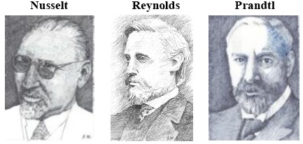
Perhaps, for the first time, students will see the utility and generality of empirical equations in convection heat transfer when dimensionless numbers are used. They will take two curves from the water tunnel experiment and two curves from the wind tunnel experiment and cast the primitive variables in these four curves into Nu, Re, and Pr dimensionless numbers and end up with a single curve with a single empirical equation that agrees very nicely with the equation in their heat transfer textbook.
Experiment 20
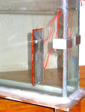
Natural Convection – Vertical Plate in Water
In addition to the Reynolds, Nusselt and Prandtl numbers presented and used in the previous experiment (Experiment 19), a new dimensionless number is presented: the Rayleigh number (Ra). Data are provided for a vertical plate with an internal electric heater undergoing natural convection cooling in water. When students plot the results on a Nusselt-Rayleigh (Nu-Ra) plane they will see the data fall very nicely along a straight line but then abruptly depart from this line at higher Ra. The straight line data produce a laminar Nu-Ra correlation that is 1.0% off the published correlation in their heat transfer textbook. The departed data represent transition to turbulence which is covered in Experiment 22.
Experiment 21
Natural Convection with Radiation – Vertical Plate in Air
A heated copper plate undergoing transient cooling in still air is used to obtain a heat transfer correlation. The cooling is by both natural convection and radiation. The radiation component requires finding emissivity, which is determined with infrared temperature measurements. Data are collected with a digital data acquisition system over a 32 minute cooling period. Students reduce these data to obtain a Nu-Ra correlation. Additionally, the convection and radiation heat fluxes are computed and plotted which reveals a radiation component that is not insignificant even at relatively low temperatures (the average plate temperature is 99°C). This result provides good instruction in multi-mode heat transfer and may even surprise your students.
Experiment 22
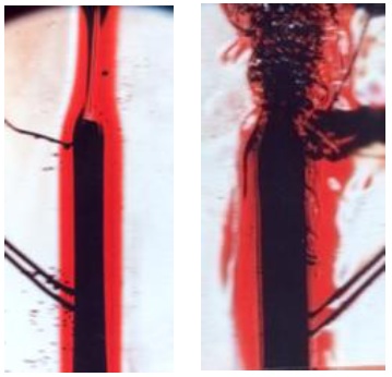
Transition to Turbulence and Flow Visualization
Laminar and turbulent flows are found in both forced and natural convection. These two flows are clearly distinct with heat transfer data from Experiment 18: Forced Convection and Radiation – Flat Plate in Air, and from Experiment 20: Natural Convection – Vertical Plate in Water. Additionally, for both experiments, we are able to visually observe and photograph laminar and turbulent flows with a schlieren optical system. The schlieren system is carefully described in the report. In the video, the alignment and adjustment of the mirrors is demonstrated. Furthermore, photos showing laminar and turbulent flows are corroborated with heat transfer data from both experiments.
Experiment 23
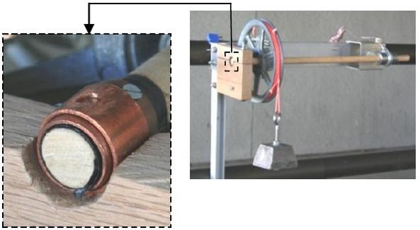
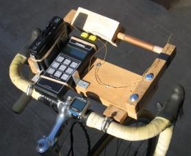
Forced Convection and Radiation – Cylinder in Crossflow
A solid copper cylinder, instrumented with a thermocouple, is mounted on a bicycle handlebar. The cylinder is first heated with a propane torch. Then, the bicycle is pedaled at constant speed, while ambient air and cylinder temperatures are read from a digital thermometer and recorded on an audio tape. The audio tape is played back to obtain temperature versus elapsed time data. These data are reduced to produce a Nusselt-Reynolds-Prandtl correlation that is 10.6% off a published correlation. Heat loss by radiation is minor, but it is accounted for by first making infrared temperature measurements to obtain the surface emissivity.
Experiment 24
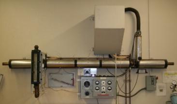
Turbulent Air Flow in a Tube
Our equipment is a concentric tube heat exchanger which accommodates heated air forced through an inner tube and cooling water that is circulated through the annular passage between the inner and outer tube. We obtain both heat transfer and pressure drop for fully-developed, turbulent air flow in the inner tube. Students reduce the data supplied to obtain a Nusselt (Nu) – Reynolds – Prandtl number correlation and a friction factor (f) – Reynolds number correlation. Compared with published correlations, the experimental Nu and f deviate by 3.5% and 10.8%.
Experiment 25
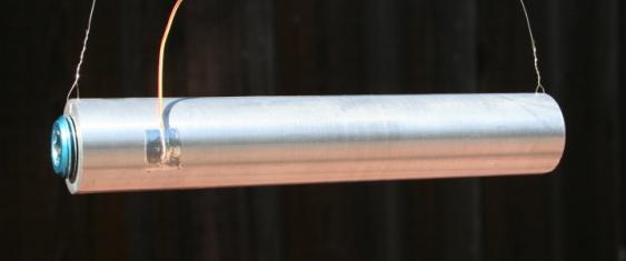
Vented and non-Vented Disk Brake Cooling Simulation
Automotive disk brake rotors for the front wheels are typically designed with internal vents to augment cooling. On the rear wheels, non-vented disk rotors are usually found. In our experiment we find the relative cooling performance of each design. Actual disk brake rotors are not used. Instead, a copper tube
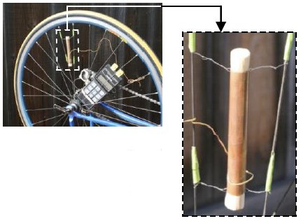
mounted between the spokes of an inverted, stationary, rear bicycle wheel is used to replicate the motion of a single vented passage. The experiments involve rotating heated tubes with the ends open and with the ends plugged, which simulate vented and non-vented rotors. Students will find the simulated, vented passage augments cooling over the simulated, non-vented passage by 40%.